“I no longer work out how to engineer a system; I work out how I make a system learn to do things. That’s a fundamental shift in engineering, biggest since the invention of fire’
Dr Aldo Faisal, Professor of AI & Neuroscience at the Dept. of Computing and the Dept. of Bioengineering at ICL
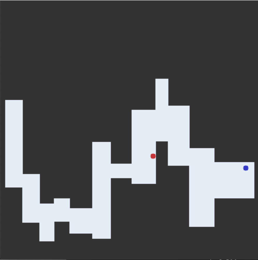
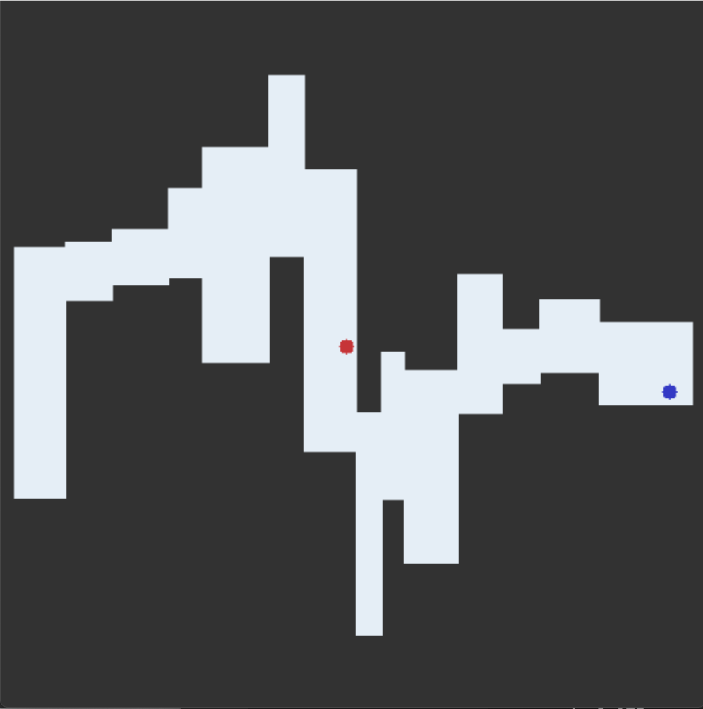
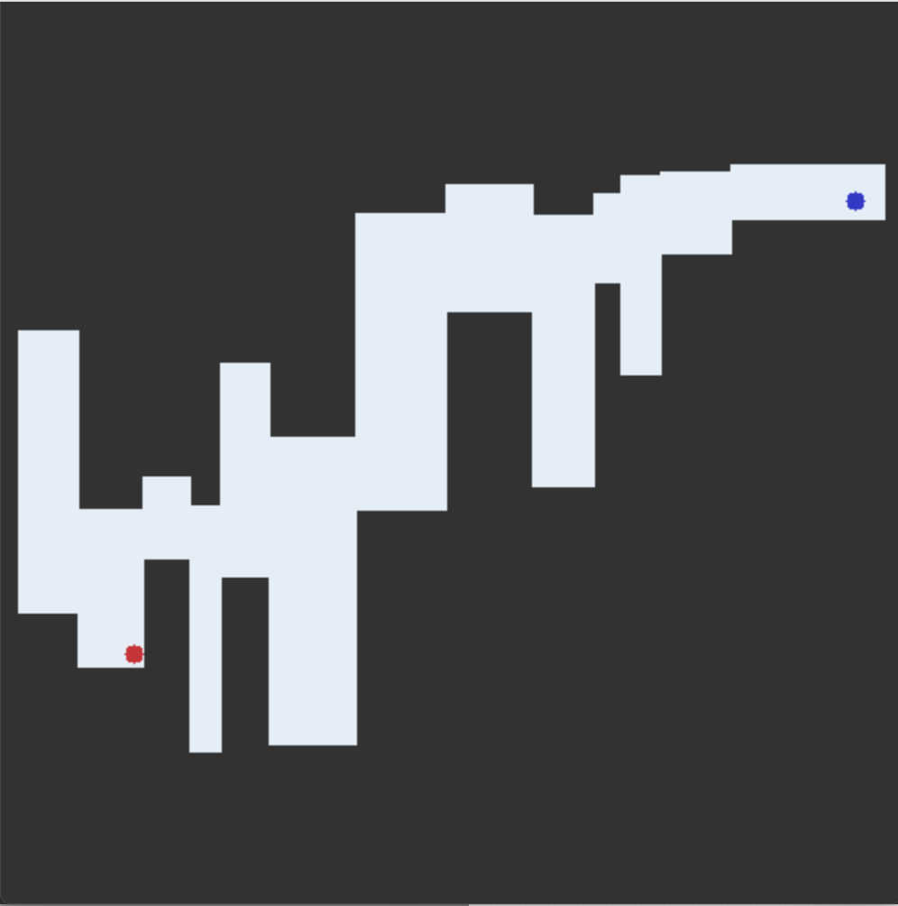
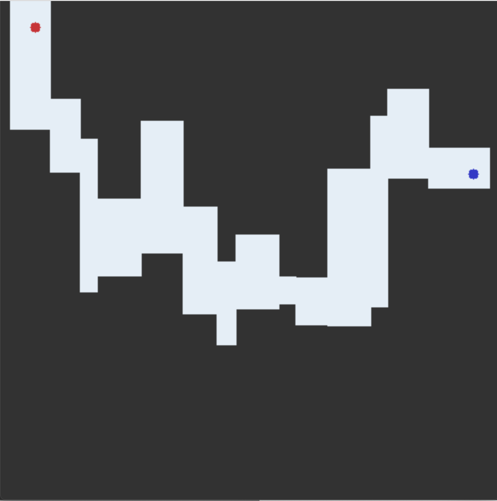
This project was created as part of a submission for Reinforcement Learning module at Imperial College London. The particular challenge tackled here focused on solving the maze environment with RL agent. The goal was to create appropriate conditions that would allow the agent (red) to learn how to get to the goal state (blue) in the maze by engineering the reward function and providing a proper pipeline of data. The theoretical side of the code was based on Markovian Decision Process and Belman Optimality Equation. An example maze environment that the agent needs to solve is presented below


RL agent solving maze.gif
The agent trains by choosing Epsilon-Greedy action at each state, which provides a balance between exploration and exploitation. At each step it takes a batch of training data from Replay Buffer and trains the neural network with it. While testing, the agent is choosing Greedy action, effectively executing the optimal path. Watch the 40 seconds gif below of the agent solving the environment
Implementation
import numpy as np
import torch
import collections
import random
import statistics

# The Network class inherits the torch.nn.Module class, which represents a neural network.
class Network(torch.nn.Module):

    # The class initialisation function. This takes as arguments the dimension of the network's input (i.e. the dimension of the state), and the dimension of the network's output (i.e. the dimension of the action).
    def __init__(self, input_dimension, output_dimension):
        # Call the initialisation function of the parent class.
        super(Network, self).__init__()
        # Define the network layers. This example network has two hidden layers, each with 100 units.
        self.layer_1 = torch.nn.Linear(in_features=input_dimension, out_features=100)
        self.layer_2 = torch.nn.Linear(in_features=100, out_features=100)
        self.output_layer = torch.nn.Linear(in_features=100, out_features=output_dimension)

    # Function which sends some input data through the network and returns the network's output. In this example, a ReLU activation function is used for both hidden layers, but the output layer has no activation function (it is just a linear layer).
    def forward(self, input):
        layer_1_output = torch.nn.functional.relu(self.layer_1(input))
        layer_2_output = torch.nn.functional.relu(self.layer_2(layer_1_output))
        output = self.output_layer(layer_2_output)
        return output

# The DQN class determines how to train the above neural network.
class DQN:

    # The class initialisation function.
    def __init__(self):
        # Create a Q-network, which predicts the q-value for a particular state.
        self.q_network = Network(input_dimension=2, output_dimension=4)
        self.target_network= Network(input_dimension=2, output_dimension=4)
        # Define the optimiser which is used when updating the Q-network. The learning rate determines how big each gradient step is during backpropagation.
        self.optimiser = torch.optim.Adam(self.q_network.parameters(), lr=0.005)
        self.optimiser_target = torch.optim.Adam(self.target_network.parameters(), lr=0.005)

    def _calculate_loss_bellman_minibatch_with_target(self, minibatch, gamma=0.9):
        #transition = (self.state, discrete_action, reward, next_state)
        #unzip the values in the minibatch
        states, actions, rewards, next_states = zip(*minibatch)

        state_tensor=torch.tensor(states, dtype=torch.float32)
        next_state_tensor=torch.tensor(next_states, dtype=torch.float32)
        action_tensor=torch.tensor(actions, dtype=torch.int64)
        reward_tensor = torch.tensor(rewards, dtype=torch.float32)
        predicted_q_value_tensor = self.q_network.forward(state_tensor).gather(dim=1, index=action_tensor.unsqueeze(-1)).squeeze(-1)
        succesor_q_value_tensor = torch.amax(self.target_network.forward(next_state_tensor),1)
        succesor_q_value_tensor = succesor_q_value_tensor.detach()
        label = reward_tensor + gamma * succesor_q_value_tensor
        loss = torch.nn.MSELoss()(predicted_q_value_tensor, label)
        return loss

    def train_q_network_bellman_minibatch_loss_with_target(self, minibatch):
        # Set all the gradients stored in the optimiser to zero.
        self.optimiser.zero_grad()
        # Calculate the loss for this transition.
        loss = self._calculate_loss_bellman_minibatch_with_target(minibatch)
        # Compute the gradients based on this loss, i.e. the gradients of the loss with respect to the Q-network parameters.
        loss.backward()
        # Take one gradient step to update the Q-network.
        self.optimiser.step()
        # Return the loss as a scalar
        return loss.item()

    def update_target_network(self):
        q_dict = self.q_network.state_dict()
        self.target_network.load_state_dict(q_dict)

class ReplayBuffer:
    def __init__(self, maxlength):
        # self.length = length
        self.replay_buffer = collections.deque(maxlen=maxlength)
        self.counter = 0
        self.x_mean = 0
        self.y_mean = 0
        # self.batch_size = size

    def buffer_size(self):
        return len(self.replay_buffer)

    def append_transition(self, transition):
        self.replay_buffer.append(transition)
        self.counter += 1
        size = len(self.replay_buffer)
        if self.counter % 200 == 0:
            x_list=[]
            y_list=[]
            for x, y, b ,n in self.replay_buffer:
                x_list.append(x[0])
                y_list.append(x[1])

            self.x_mean = statistics.mean(x_list)
            self.y_mean = statistics.mean(y_list)
            # print('X: '+ str(x_mean) + 'Y: '+ str(y_mean))
        return self.x_mean, self.y_mean, size


    def rand_mini_batch(self, size):
        # minibatch_indices = np.random.choice(range(len(self.replay_buffer)), size)
        # print(minibatch_indices)
        minibatch=[]
        if len(self.replay_buffer) > size:
            minibatch_indices = np.random.choice(range(len(self.replay_buffer)), size)
            for i in range(size):
                minibatch.append([])
        else:
            minibatch_indices = np.random.choice(range(len(self.replay_buffer)), len(self.replay_buffer))
            for i in range(len(self.replay_buffer)):
                minibatch.append([])
        # print(minibatch_indices)
        for i in range(len(minibatch)):
            index = minibatch_indices[i]
            minibatch[i]=np.array(self.replay_buffer[index])

        return minibatch
##########################################################################################
##                                                                                      ##
##                                  A G E N T                                           ##
##                                                                                      ##
##########################################################################################

class Agent:

    # Function to initialise the agent
    def __init__(self):
        # Set the episode length
        self.episode_length = 500
        # Reset the total number of steps which the agent has taken
        self.num_steps_taken = 0
        # The state variable stores the latest state of the agent in the environment
        self.state = None
        # The action variable stores the latest action which the agent has applied to the environment
        self.action = None
        self.dqn = DQN()
        self.dqn.update_target_network()
        self.buffer = ReplayBuffer(maxlength=5000)
        self.reward = None
        self.episode_counter = -1
        self.training = True
        self.greedy_run = True
        self.last_greedy_run_score = 66

    # Function to check whether the agent has reached the end of an episode
    def has_finished_episode(self):
        if self.num_steps_taken % self.episode_length == 0:
            self.num_steps_taken = 0
            self.greedy_run = not self.greedy_run
            if not self.greedy_run:
                self.episode_counter += 1
            if self.greedy_run:
                self.episode_length = 100
            return True
        else:
            return False

    # Function to get the greedy action for a particular state
    def get_greedy_action(self, state):
        #
        state_tensor=torch.tensor(state).unsqueeze(0)
        discrete_action = torch.argmax(self.dqn.q_network.forward(state_tensor)).item()
        action = self._discrete_action_to_continuous(discrete_action)
        return action

    def get_greedy_action_discrete(self, state):
        #
        state_tensor=torch.tensor(state).unsqueeze(0)
        discrete_action = torch.argmax(self.dqn.q_network.forward(state_tensor)).item()
        return discrete_action

    def get_epsilon_action(self):
        # epsilon greedy function
        episode = self.episode_counter
        steps = self.num_steps_taken
        # decay of epsilon over episodes
        eq = 1 * 0.95 ** episode
        if 25 > episode > 15:
            self.episode_length = 300
            epsilon = 0.1
        elif episode == 0:
            self.episode_length = 2000
            epsilon = 1
        else:
            self.episode_length = 500
            epsilon = eq
        if random.uniform(0,1) > epsilon:
            state_tensor=torch.tensor(self.state).unsqueeze(0)
            action = torch.argmax(self.dqn.q_network.forward(state_tensor)).item()
        else:
            action_list = [0]*35 + [1] *30 +[3] * 30 + [2] * 5
            action = random.choice(action_list)
            # action = random.randint(0,3)
        return action, epsilon, episode

    def _discrete_action_to_continuous(self, discrete_action):
        #NESW 0,1,2,3
        if discrete_action == 0:
            # right
            continuous_action = np.array([0.02, 0], dtype=np.float32)
        elif discrete_action == 1:
            # up
            continuous_action = np.array([0, 0.02], dtype=np.float32)
        elif discrete_action == 2:
            # Move left
            continuous_action = np.array([-0.02, 0], dtype=np.float32)
        elif discrete_action == 3:
            # Move down
            continuous_action = np.array([0, -0.02], dtype=np.float32)
        return continuous_action

        # Function to get the next action, using whatever method you like
    def get_next_action(self, state):
        self.state = state
        # Choose the next action.
        if self.greedy_run == True or not self.training:
            discrete_action = self.get_greedy_action_discrete(state)
            # print("GREEDY RUN" + " episode: " + str(self.episode_counter+0.5) + " step " + str(self.num_steps_taken))
        else:
            discrete_action, epsilon, episode = self.get_epsilon_action()
            # print('epsilon: '+ str(round(epsilon,3))+' episode: '+ str(episode)+' step: '+ str(self.num_steps_taken))
        # Store the action; this will be used later, when storing the transition
        self.action = discrete_action
        # Convert the discrete action into a continuous action.
        action = self._discrete_action_to_continuous(discrete_action)
        # Update the number of steps which the agent has taken
        self.num_steps_taken += 1

        return action

    # Function to set the next state and distance, which resulted from applying action self.action at state self.state
    def set_next_state_and_distance(self, next_state, distance_to_goal):
        # Reward function, containing reducing condition if the chosen action lead to hitting the wall
        reward = 0.2*(2**(1/2) - distance_to_goal)**2
        if self.state[0] == next_state[0] and self.state[1] == next_state[1]:
            reward = reward - 0.005

        transition = (self.state, self.action, reward, next_state)

        if self.greedy_run:
            self.last_greedy_run_score = distance_to_goal
            if distance_to_goal < 0.03:
                self.training = False

        if not self.training :
            print("Training stopped!" + " greedy_score: " + str(self.last_greedy_run_score) )
        elif self.greedy_run:
            print("run run run!" + " greedy_score: " + str(round(self.last_greedy_run_score,4)))
        else:
            # adding transition to buffer
            x_mean, y_mean, size = self.buffer.append_transition(transition)
            print("reward: " + str(round(reward,3))+" x_mean: " + str(round(x_mean,3))+ " y_mean: " + str(round(y_mean,3))+ " size: " + str(size)+ " greedy_score: " + str(round(self.last_greedy_run_score,4)))

            #get minibatch from buffer if there's enough samples there
            if self.buffer.buffer_size() >= 100:
                minibatch = self.buffer.rand_mini_batch(2000) #+ int(self.num_steps_taken/100)
                loss_value = self.dqn.train_q_network_bellman_minibatch_loss_with_target(minibatch)

            if self.num_steps_taken%500 == 0:
                self.dqn.update_target_network()

    def training_finished(self):
        return self.training
The implemented solution for solving the maze environment is Deep Q-Learning with Replay Buffer and Target Network. It additionally contains an evaluation check after each training episode that can stop the training given the agent reaches the goal with greedy policy. The hyper parameters were hand-tuned using trial and error method combined with understanding of the underlying principles. Alternative implementation included a variation of Prioritised Experience Replay, however it was found that it actually worsen the performance of the network due to added computational complexity. The implementation is outlined below.
Lines 8-24 contain Network class. This class allows for initiation of the neural net- work with given architecture using torch module. Additionally, the forward function is defined which is responsible for gaining network’s output given an input.
Lines 27-68 contain DQN class. This class is responsible for training of the neural net. The two instances of the Network class are initiated with respective optimisers, the regular q network and the target network. Further functions are responsible for calculation of the loss and its back-propagation. The mean-square-error loss of the mini-batch is calculated using Bellman equation, with incorporated target network for successive state-action value prediction.
Lines 70-116 contain ReplayBuffer class. This class allows for creation of container where the agent’s transition will be put into. It contains methods for appending the transition to the buffer (container) and for sampling of random mini-batch for training purposes.
Lines 123-260 contain the main body of code in form of Agent class. Firstly, the instances of DQN and ReplayBuffer are initiated, along with multiple numerical and flag variables. Function ”has finished episode” is responsible for checking whether the episode is done and additionally it initiates the greedy run evaluating the policy every other episode. Function ”get greedy action” calculates the greedy action by taking the argmax on forward pass through neural. Function ”get epsilon function” can either return the greedy function, with the same mechanism as the previously mentioned function, or a randomized action. The randomized action has respectively 35, 30, 30 and 5 percent chance of being right, up, down and left. This distribution favorizes actions leading to the goal state. Epsilon is decaying with the number of episodes, in order to ensure high exploration at the start of training and then higher specialization in getting the right values for optimal path states. The function ”get next action” checks whether the agent is in training or evaluation mode and then the respective epsilon-greedy or greedy action is gotten. The function ”set next state and distance” is responsible for training of the agent. Firstly, it calculates the reward based on the supplied distance to goal. The reward function was tuned to give better value differentiation near the initial state. Next, if the agent is in training mode, the transition is appended to the buffer and a mini-batch is randomly sampled from it. Based on that batch, the prediction loss is calculated and back propagated through network for learning. Finally, the target network is updated with set frequency.
